
~Minimax, three ways
This is a short technical note written in the process of working out some definitions for a paper about using an approximate minimax regret training objective to mitigate goal misgeneralisation in advanced deep reinforcement learning systems. I define a minimax objective in three different ways, and show that the definitions are equivalent under certain assumptions.
Thanks to my colleagues Karim Abdel Sadek and Michael Dennis for helping me understand the necessary game theory and decision theory to figure this out.
§Background
In the aforementioned paper, we study the generalisation properties of approximate optima under different objectives. We want to study approximate optima, rather than exact optima, because the former is more like what our training methods will find in practice.
However, one of the objectives we want to study is minimax regret, which is an objective that actually involves two optimisers: we want to take the minimum of a function that involves a maximum. It wasn’t immediately obvious to me what the appropriate approximate relaxation was for this type of adversarial optimisation.
My colleagues and I came up with a few candidate definitions. I got to work trying to prove they were equivalent in some appropriate sense. I got stuck, so I retreated to the exact case, reasoning that if I can understand how the definitions relate to each other in the exact case, then I should be in a better position to understand the relationships between the approximate relaxations.
This note doesn’t discuss what regret is. It’s not really important for today—we’re just interested in the minimax part. I also don’t discuss why we are interested in minimax regret as an objective. For more background, see the paper (when it comes out), or this old essay by Savage (1951) that abstracted minimax regret as a general principle for making decisions under uncertainty from the statistics literature.
This note also doesn’t much discuss the approximate relaxations. Here I’m just writing out the proofs from the exact case, partly as a way of checking my work, and partly because I think the proofs are pretty neat.
Update: For the approximate case, see this sequel note.
§Three formal definitions…
Suppose we have a function . As I said, it doesn’t matter what the function represents. It also doesn’t matter much what the sets and are. All we really need to know is that we want to find a first argument so as to minimise the maximum possible value for any value of the second argument . (The only assumption I make on , , and is that all the maxima and minima I refer to exist.)
Such abstraction is sufficiently cumbersome that I would prefer to use slightly more concrete terminology. The symbols are chosen to suggest that is the regret from taking action when the world is in state . The objective would then be phrased, we want to find an action that minimises the maximum regret under any world state.
The question is, how should we formalise this objective? Here are three ways.
§§The standard definition from decision theory
The first is the standard decision theory definition, and is a straightforward transliteration of the above description:
Definition 1: An action is minimax(1) if
While this definition is straightforward, it’s difficult to see how to replace the maximiser with an approximate version, since it’s nested inside a minimum.
§§The standard definition from game theory
In an attempt to address this shortcoming, we appeal to game theory, where we find plenty of tools for studying competition between optimisers:
Definition 2: An action is minimax(2) if there exists such that both
This condition says that is a Nash equilibrium of a two-player, zero-sum game where the first player selects an action and the second player selects a state , respectively aiming to minimise or maximise the regret . A minimax(2) action is then any action that is part of a Nash equilibrium.
It’s easy to see how to relax this definition: just replace both of the constraints with approximate version, effectively permitting each player a small incentive to change strategy (making it a near-Nash equilibrium).
However, not all games have Nash equilibria, or even near-Nash equilibria. For example, suppose for some reason we want to find a pure strategy equilibrium rather than a mixed strategy equilibrium. It is well-known that some games lack a pure strategy equilibrium (e.g., rock/paper/scissors). Moreover, even for mixed strategies, if the strategy space is not compact, there may not be a Nash equilibrium.
In such cases, minimax(2) is not well defined. In contrast, minimax(1) is well-defined for any , , as long as the maxima and minima exist. Intuitively, we don’t need there to be an equilibrium for us to be able to talk about minimising the worst possible response.
§§An alternative definition
This brings us to the third definition, which, as far as I can tell, is not a standard way of defining minimax, but has the potential to capture the nice properties of both minimax(1), namely not relying on an equilibrium, and of minimax(2), namely separating out the maximiser and the minimiser so that each can be relaxed.
Definition 3.1: A max map is any function such that for all ,
Definition 3.2: Let be any max map. An action is minimax(3) if
This definition is not as straightforward as the previous ones. Let’s unpack it. Note that this definition depends on a choice of a max map that has the specified property. Intuitively, represents a model of a deterministic, worst-case response to every possible action .
Given a max map , we then define minimax(3) actions by optimising the single-argument function . Compared to definition 1, we factor out the inner optimisation problem into computing the max map. Compared to definition 2, it’s like we’re playing a game in our head against a model of a particular optimal adversary, rather than playing a real game against a real adversary.1,2
What we gain from the extra complexity is the following. Like minimax(1), minimax(3) is well-defined even if the zero-sum game has no Nash equilibrium. Moreover, like minimax(2), we can clearly relax both the maximisation (by relaxing the condition on the max map ) as well as the minimisation (by relaxing the condition on the action ).
§… and their equivalence
Of course, it remains to prove that this definition actually captures the same kinds of actions as the other two. As a starting point, we also prove to ourselves that the first two definitions are equivalent to each other (this is a well-known result, but I am interested in the proof).
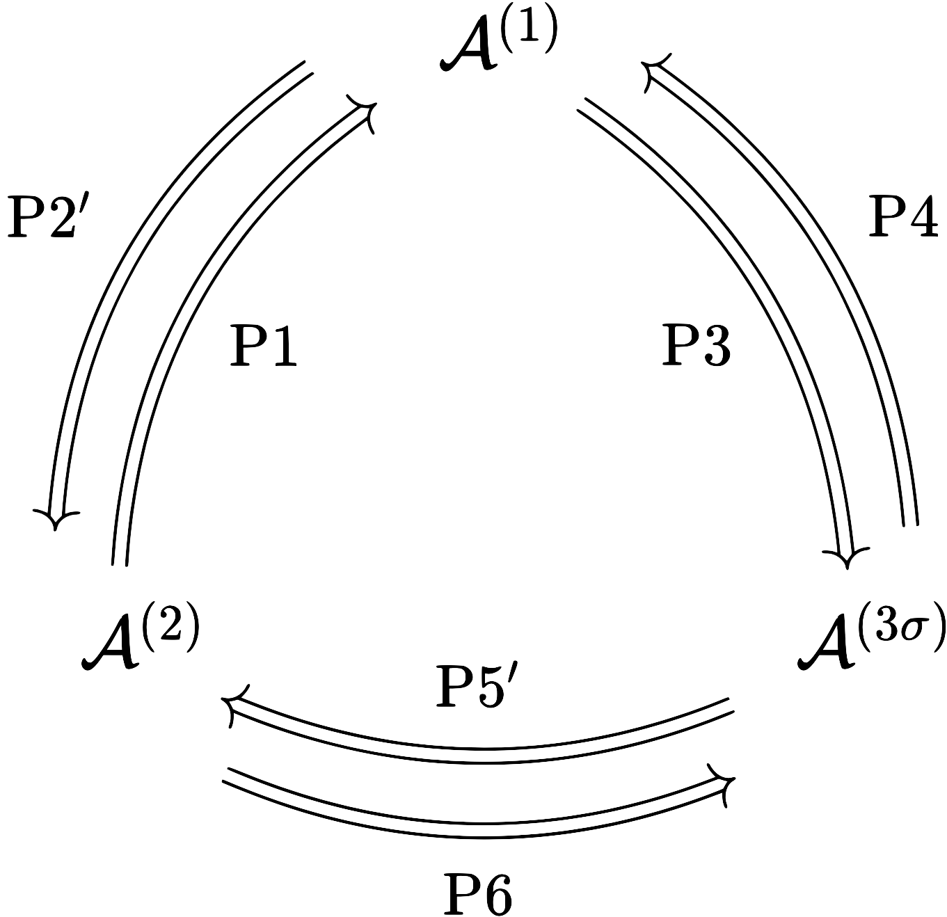
The following diagram summarises the equivalences between the three definitions. The symbols , , and represent the conditions minimax(1), minimax(2), and minimax(3), respectively. P1 through P6 indicate numbered propositions establishing each relationship. P2 and P5 are primed because these relationships involve an additional assumption (that an equilibrium exists).
§§Aside: The max–min inequality and equilibria of zero-sum games
Before we prove these equivalences, we take a brief detour into some basic properties of zero-sum games. First, we note the following inequality that holds for any function and any sets , (as long as the minima and maxima exist; though in this case if they do not, the lemma holds with infima and suprema instead).
Lemma 1 (max–min inequality):
Proof. Let and let . Then we have
We will also need the following, related result, which says that, if our zero-sum game has an equilibrium, then the max–min inequality is an equality. (The converse also holds, but we do not need it for this note.)
Lemma 2: Suppose there exists such that and . Then
Proof. We already know from lemma 1 that LHS RHS. Under these conditions we also have LHS RHS as follows:
Intuitively, lemma 1 says that if the minimiser chooses their action as a function of the state, they will always do at least as well as if they must choose a constant action without knowledge of the state. Lemma 2 then says that an equilibrium can only exists when the minimiser can do no better by choosing their action with (vs. without) knowledge of the strategy of the maximiser, and vice versa.
I really like the symmetry in these two proofs. Notice that the sequence of terms we relate is the same in both cases, we just somewhat reorder the definitions we apply to them and how we relate them with inequalities or equalities. Neat!
Remark. Lemmas 1 and 2 are some basic results that are related to the famed minimax theorem of von Neumann that was the foundation of game theory.
Von Neumann proved that the max–min inequality is an equality for all two-player zero-sum games with mixed strategies over finite action spaces. (Since that time, minimax theorems have been proven for more general classes of functions). Lemma 1 shows the trivial side of this equality, which holds for all functions as long as min and max are defined (and beyond).
It’s also true that, if the max–min inequality is an equality, then an equilibrium exists. Therefore, von Neumann’s minimax theorem showed that all discrete zero-sum games with mixed strategies have equilibria. Lemma 2 is the converse: if an equilibrium exists, the max–min inequality is an equality.
Proving a minimax theorem requires some more advanced techniques, and certain assumptions on the function and the sets. Luckily, for this note we can bypass such details by just assuming an equilibrium exists.
§§Equivalence of minimax(1) and minimax(2)
Now, we are ready to prove the equivalence of definitions 1 and 2. First, we show that minimax(2) implies minimax(1). For this direction, we implicitly assume that an equilibrium exists (in supposing that minimax(2) holds), so we don’t have to worry about the case where there are no equilibria in the zero-sum game.
Proposition 1: Let be minimax(2). Then is minimax(1).
Proof. Suppose is minimax(2). So, there exists such that both and . Then, In summary, . Observe, the LHS of this inequality is part of the minimisation operation on the RHS. Therefore, we must have an equality, and is a minimiser or the operand on the RHS. Therefore, we have the minimax(1) condition
Notice that, while the max–min inequality is an equality under these assumptions (by lemma 2, and also very nearly a byproduct of this proof), we only needed the inequality this time. This is a good sign, because when it comes to the approximate case, we would only want to assume that there is an approximate equilibrium without additionally making the stronger assumption that there also exists an exact equilibrium.
Now, for the converse direction. This direction can’t hold if the zero-sum game has no equilibria: then we can have a minimax(1) action but there are no minimax(2) actions. However, we prove that this is the only case in which the converse doesn’t hold: as long as the zero-sum game has an equilibrium, then, by lemma 2, the max–min inequality is an equality, an equilibrium exists, and the minimax(1) action is part of an equilibrium.
Proposition 2: Suppose there exists some that is minimax(2). Let be minimax(1). Then is minimax(2).
Proof. To say there exists an that is minimax(2) is the same as saying an equilibrium exists, so lemma 2 applies. Let be minimax(1), we have . Let . Then we have The first and final terms are equal. Therefore, the two inequalities must be equalities. Each gives us part of the minimax(2) condition,
This proof is cute in that it packages together the proof of both minimax(2) conditions into one chain of relations. The structure is also very similar to the structure of the proof of proposition 1. The text after the “summary” in that proof essentially appends “ (by definition of min)” to the end of the chain of relations. Then both proofs are based on the same ‘cycle’ of terms. Based on the different assumptions, different relations are replaced with inequalities. But once we complete the cycle, it becomes clear that all the terms are actually equal. I think that’s pretty neat.
§§Equivalence of minimax(1) and minimax(3)
OK. So far so good, but that was all very standard game theory. Now let us turn to the more interesting cases involving the new, alternative definition! We’ll start by showing that minimax(1) and minimax(3) are equivalent.
When I say “minimax(3),” I’m leaving unspecified. I mean we should be able to take any that meets the condition in the definition, and prove that the equivalence holds for the version of the definition specific to that . That means the below statements and proofs need to be conditioned on .
Proposition 3: Let be any max map. Let be minimax(1). Then is minimax(3).
Proof. Suppose is minimax(1). So, we have . Then, This suffices to prove the minimax(3) condition:
Note that for the inequality, we actually have an equality by definition of . However, all we need is the inequality to establish that is a minimiser. It wouldn’t matter here if we used the equality instead, but when it comes time to relax to the approximate case, we don’t want to use the definition of more than we have to, because each time we use it we introduce an approximation error.
Now, for the converse. Once again, the proof is highly symmetrical to the previous one.
Proposition 4: Let be any max map. Let be minimax(3). Then is minimax(1).
Proof. Suppose is minimax(3). So, we have . Then, This suffices to prove the minimax(1) condition:
The final step is a little more subtle than previous invocations of the definitions of max and min. We’re using the fact that for all , simultaneously. Increasing the operand of the minimum everywhere may change the minimising argument, but it can’t decrease the value of the minimum. Note, again, that we actually have an equality here by definition of . However, we can get away with only an inequality, which should pay off in the approximate case.
§§Equivalence of minimax(2) and minimax(3)
It follows from propositions 1, 2, 3, and 4 that minimax(2) and minimax(3) are also equivalent (for any , when an equilibrium exists). So, we are done!
However, when it comes time to relax these definitions into approximate versions, following each of these equivalence proofs will involve introducing approximation errors as we go. The best results will come from the most direct relationship between the definitions, in particular using each approximation condition as few times as possible. Therefore, it is also of interest to write out the direct proofs that minimax(2) and minimax(3) are equivalent, to make sure there is no redundancy in the argument.
Let’s complete the picture by studying the relationship between these conditions directly, starting by proving that minimax(3) implies minimax(2):
Proposition 5: Let be any max map. Suppose there exists some that is minimax(2). Let be minimax(3). Then is minimax(2).
Proof. Suppose is minimax(3). That is to say, . We want to show there exists some in equilibrium with . Let’s start by taking . It follows that Since the first and final terms are equal, all of the inequalities are equalities. The first and the last give us the two parts of the minimax(2) definition,
This proof neatly blends together the chains of relations from propositions 2 and 4. For example, note the two uses of the definition of max as in the proof of proposition 4 (one on the inside of a min operator); and note the use of lemma 2 as in proposition 2. Moreover, there is no obvious redundancy in the argument, since each assumption on , , or is used exactly once. Therefore, this proof seems suitably direct.
Finally, we prove that minimax(2) implies minimax(3).
Proposition 6: Let be any max map. Let be minimax(2). Then is minimax(3).
Proof. Suppose is minimax(2). Then there exists such that both and . It follows that This suffices to prove the minimax(3) condition:
Similarly, this proof is reminiscent of the proofs of propositions 1 and 3. For example, note the use of the max–min inequality. Once again, we only use each definition once, so it seems suitably direct. We’re also taking the reversed route around the same cycle of terms that arose in proposition 5.
§Conclusion
Thus, the new definition is equivalent to the old ones after all. As I said, I think these proofs are pretty neat. Moreover, they’re going to help me define the thing we are actually interested in, which is an approximate notion of minimax optimisation. Speaking of which, I had better get back to work on that…
Update: For the approximate case, see this sequel note.
Karim Abdel Sadek noted that definition 3 is reminiscent of a game theoretic equilibrium concept from a sequential game, where one can consider strategies to be functions that a player would use to decide their particular action in any given part of the ‘game tree.’↩︎
Definition 3 also seems conceptually reminiscent of Skolemisation from first-order logic, whereby we transform a formula with an existential quantifier by introducing a function that maps each universally quantified variable to a particular constant, yielding an equisatisfiable formula, as in the example ↩︎