Everyone seems to be talking about the paper by Finzi et al. (2026), “From Entropy to Epiplexity: Rethinking Information for Computationally Bounded Intelligence.” I finally got around to studying it this week.

In this short technical note, I discuss the theoretical definition of epiplexity from a computer science perspective, work through some of the basic examples and properties from the paper in a slightly generalised setting, and then explore various examples of my own.

Disclaimer: This note will be exclusively focused on the formal theoretical framework of defining epiplexity within a minimum description length framework, as a kind of successor to (algorithmic) information theory. There is a whole second side of this paper that is about applying this framework as a lens on deep learning “paradoxes” and phenomena. I am still reading that part, I might write some thoughts on it later, but I won’t discuss it in this note.

Acknowledgements: Thanks to Joan Velja and Lennie Wells for helpful discussions.

Word count: 5625

Contents:

• Defining epiplexity
  • Setting and overview
  • Computable probability distributions
  • Representing resource limits
  • The optimal two-part code
  • Epiplexity
  • Time-bounded entropy, or “epientropy”
  • Visualising the definitions
• Examples and basic properties of epiplexity
  • Uniform distribution
  • General upper bounds
  • Relaxing the restrictions
• Recovering unbounded complexity and entropy
• Independent sequences
  • Iterating variables
  • Iterating probabilistic models
  • A basic upper bound
  • Weighted minimum description length
  • Allowing more programs
• Breaking ties
  • What are ties?
  • Toy example of a tie
  • Why break for less structure?
  • Alternative tie-breakers
  • Dissolving the tie
• Conclusion

§Defining epiplexity

Epiplexity is billed as “the structural content in data,” a complexity or information measure that excludes any information that appears to be randomness to a learner/observer with limited computational resources. That sounds useful, let’s see how it’s formalised.

§§Setting and overview

Let’s view the data as a binary random variable $X \in \{{\tt 0},{\tt 1}\}^{n}$ for some fixed number of bits $n \in \mathbb{N}$. This random variable has some probability distribution, call it $Q \in \Delta(\{{\tt 0},{\tt 1}\}^{n})$.

The way I see it, there are two core motivating ideas behind epiplexity:

1. The first idea is that there might be some “structure” in the distribution $Q$ leading to patterns in $X$ that render some of the bits predictable in terms of others. It would be nice to be able to quantify how much of $X$ is predictable based on these kinds of patterns, versus unpredictable entirely.

   The paper’s approach is broadly to consider compressing $X$ in two parts: first encoding a program representing a probability distribution, and second encoding $X$ itself with the optimal coding scheme for that probability distribution. If program is well-chosen this could be cheaper than coding $X$’s bits directly, and we can call the bits spent on coding the program structural information (the remaining bits are a kind of entropy).

2. The second idea is that some patterns in $X$ that could be used to more efficiently compress it in principle might in practice be out of reach for an observer with computational limits. For example, a cryptographically secure PRNG emits very structured data (in fact it’s deterministic) and this structure is easy enough to describe with a short program, but the fastest program to exploit this structure to design a coding scheme is going to have an unreasonably long run-time.

   The paper’s response is to repeat step (1) but considering only programs that fit within a particular computational budget (specifically, a time complexity budget).¹ The epiplexity is the length of the shortest efficient program that encodes a probability distribution used in an optimal coding scheme, where optimality is judged among coding schemes based only on other efficient-program-based probability distributions. If the time budget doesn’t allow detecting a cryptographically secure PRNG, then its output bits may as well be random, and will contribute to the (time-bounded) entropy, rather than the epiplexity.

Epiplexity is short for “epistemic complexity,” with “epistemic” indicating the definition is relative to the observer’s resource constraints.

That was fast—let’s go through it again in much more detail.

§§Computable probability distributions

Let’s formalise what it means for a program to represent a probability distribution. The two fundamental operations an observer might want to use to interact with a probability distribution are sampling (useful for generation) and density estimation (useful for computing cross entropy training loss and designing optimal codes).

Fix a prefix-free universal Turing machine $U$.² Then, a (computable) probabilistic model on $\{{\tt 0},{\tt 1}\}^{n}$ is any program ${\tt P}$ for $U$ that supports access to a probability distribution via these two fundamental operations.

• Density evaluation: Let $x \in \{{\tt 0},{\tt 1}\}^{n}$. We require that simulating ${\tt P}$ on the input ${\tt 0} x$ via $U$ halts, producing as output a finite-precision number $P_{{\tt P}}(x)$.³ We further require that the function $P_{{\tt P}}$ satisfies the properties of a probability mass function:

  • For all $x \in \{{\tt 0},{\tt 1}\}^{n}$, $P_{{\tt P}}(x) \in [0,1]$.

  • $\sum_{x \in \{{\tt 0},{\tt 1}\}^{n}} P_{{\tt P}}(x) = 1$.

• Sampling: Let $u \in \{{\tt 0},{\tt 1}\}^\infty$ be an unbounded string of uniformly random noise. We require that simulating ${\tt P}$ on input ${\tt 1} u$ halts, producing the string $x \in \{{\tt 0},{\tt 1}\}^{n}$ with probability $\mathbb{P}_ {\tt P}(x)$.

Of course, we also require that the two operations match in terms of the underlying probability distribution, that is, for all $x \in \{{\tt 0},{\tt 1}\}^{n}$, $$P_{{\tt P}}(x) = \mathbb{P}_ {\tt P}(x).$$

Note that there are three P symbols floating around:

1. ${\tt P}$ is a program for our universal Turing machine, specifically a computable probabilistic model. It’s a binary string. (The paper uses the notation $\mathrm{P}$.)
2. $P_{{\tt P}}$ is the density function encoded by the program ${\tt P}$. It’s a function mapping each binary string to its probability mass. (The paper uses the notation $\mathrm{Prob_P}$ or italic $P$.)
3. $\mathbb{P} _ {\tt P}$ is the probability of generating a string under the sampler encoded by the program ${\tt P}$, given uniform random noise input (The paper uses the slightly cumbersome notation $\mathrm{Pr}_ {u\sim U_\infty}[\mathrm{Sample_P}(u)=\cdot]$, which I elected to streamline)

Fortunately, we only need to keep (1) and (2) around going forward, since we agreed by definition that $P_{{\tt P}}= \mathbb{P}_ {\tt P}$.

§§Representing resource limits

The above definition of a probabilistic model is similar to Definition 7 from the paper. However, unlike the paper’s Definition 7, we haven’t yet introduced any restrictions on the probabilistic models to represent the observer’s limited computational affordances.

The paper focuses on time complexity, and defines a time-bounded families of probabilistic models $\mathcal{P}_T$ where $T$ is some time-limit function (of $n$) telling us how many steps of $U$ are allowed to be used by ${\tt P}$ during density evaluation or sampling.

In this note, I wanted to step back and define computable probabilistic models in general, so that I can talk about restricting to arbitrary sets of probabilistic models over $\{{\tt 0},{\tt 1}\}^{n}$. Therefore, below, I’ll consider a generic set of allowed probabilistic models, denoted $\mathcal{P}$. This set could be defined by a time bound (like $\mathcal{P}_T$). Alternatively, it could be a finite set of hand-constructed programs, or the set of all computable probabilistic models, for example.

This generalisation is an extension mentioned but not pursued in the paper. I adopt it in this note because for the basic properties we consider the extensions are immediate, and it also allows greater flexibility in exploring connections to other topics in (algorithmic) information theory.

§§The optimal two-part code

The next step towards defining epiplexity is to develop the two-part coding scheme for efficiently compressing the random variable $X$, subject to our computational limits.

Suppose our observer wants to store an instantiation of $X$ using a probabilistic model ${\tt P}\in \mathcal{P}$, namely via the following scheme:

1. First, they encode the probabilistic model ${\tt P}$.

   Since ${\tt P}$ is a program, they can store the bits directly, costing $\text{len}({\tt P})$ bits.

2. Second, they use an optimal code algorithm to design a code for samples from the distribution $P_{{\tt P}}$, and then use this code to encode the instantiation of $X$ itself.

   The cost in bits will depend on the exact value of $X \sim Q$. In expectation, the cost will be the cross entropy of $P_{{\tt P}}$ relative to $Q$, $\mathbb{E}_{X \sim Q}\!\left[-\log_2 P_{{\tt P}}(X)\right]$.⁴

The total number of bits the observer can expect to store if they use ${\tt P}$ for encoding $X$ is therefore $$L(X; {\tt P}) = \text{len}({\tt P}) + \mathbb{E}_{X \sim Q}\!\left[-\log_2 P_{{\tt P}}(X)\right],$$ which we call the description length of $X$ via ${\tt P}$.

Is this a good way of compressing a random value? That depends. If $P_{{\tt P}}\approx Q$, then the optimal coding scheme will allow the observer to store $X$ almost as efficiently as if they knew $Q$, which could be very efficient in some cases. Either way, they also need to store ${\tt P}$, so that the decompressor can reconstruct the coding scheme used to encode $X$ to decode it at the other end.

Fortunately, the observer gets to choose which probabilistic model ${\tt P}$ to use, at least within the limits of their computational resources. As promised, let’s denote the set of probabilistic models available to our observer as $\mathcal{P}$ (this might be all computable probabilistic models, or just efficient ones, or whatever). The observer can then choose ${\tt P}$ so as to make $P_{{\tt P}}$ as close to $Q$ as possible, while balancing bits saved encoding $X$ against the bits they have to add to encode ${\tt P}$ alongside it. The best they can do is $$L_\mathcal{P}(X) = \operatornamewithlimits{\vphantom{arg\,}min}_{{\tt P}\in \mathcal{P}} L(X; {\tt P}) = \operatornamewithlimits{\vphantom{arg\,}min}_{{\tt P}\in \mathcal{P}} \big\{ \text{len}({\tt P}) + \mathbb{E}_{X \sim Q}\!\left[-\log_2 P_{{\tt P}}(X)\right] \big\},$$ which we’ll call the ($\mathcal{P}$-restricted) minimum description length of $X$.⁵

§§Epiplexity

Finally, we are in a position to define epiplexity itself.

Given $X \sim Q$, the ($\mathcal{P}$-restricted) epistemic complexity, or epiplexity of $X$, denoted $S_\mathcal{P}(X)$, is simply the length of the (shortest) program from a two-part code achieving the minimum description length. Formally, $$S_\mathcal{P}(X) = \text{len}({\tt P}_\star) \quad \text{such that} \quad {\tt P}_\star \in \operatornamewithlimits{arg\,min}_{{\tt P}\in \mathcal{P}} \big\{ \text{len}({\tt P}) + \mathbb{E}_{X \sim Q}\!\left[-\log_2 P_{{\tt P}}(X)\right] \big\}$$ (breaking ties by lowest $\text{len}(\cdot)$).⁶

Recall that epiplexity was billed as the structural information in data accessible to a computationally bounded observer. In summary:

• By using the two-part code, we decomposed the information in $X$ into that required to describe the computation of a density (structural information) and the remaining information.

• By searching for the shortest overall description length, we extracted as much structure as possible into the program part, right up until the point where further bits added to the program stopped saving more than an equal number of bits of cross entropy.

• By restricting ourselves to programs in $\mathcal{P}$ for the encoding, we account for only computable structure that the observer can actually afford to use. The bits remaining may or may have structure, but if they do, it’s structure that is beyond the observer’s computational resources to exploit.

§§Time-bounded entropy, or “epientropy”

This brings us to the complementary notion introduced in the paper: what about the bits the observer expects to use to compress $X$ during the second part of the optimal two-part code? These bits represent the remaining, apparently-random information content of $X$ that wasn’t explained by affordable computational structure.

Formally, I’m referring to the quantity $H_\mathcal{P}(X)$ where $$\begin{align*} H_\mathcal{P}(X) &= \mathbb{E}_{X \sim Q}\!\left[-\log_2 P_{{\tt P}_\star}(X)\right] \\[2ex] \text{such that}\quad {\tt P}_\star & \in \operatornamewithlimits{arg\,min}_{{\tt P}\in \mathcal{P}} \big\{ \text{len}({\tt P}) + \mathbb{E}_{X \sim Q}\!\left[-\log_2 P_{{\tt P}}(X)\right] \big\} \end{align*}$$ (again, breaking ties by lowest $\text{len}(\cdot)$).

The paper calls $H_\mathcal{P}(X)$ the time-bounded entropy of $X$. However, since we’re not restricting ourselves to time-bounded program classes, we’ll need a new name.

For a full name, I think we could mirror that of epiplexity, calling it “$\mathcal{P}$-restricted epistemic cross entropy.” Just like with epiplexity, we might want to include “epistemic” to nod to the idea of the structure/randomness distinction being dependent on the (computational resources available to the) observer. We might like to include “cross” because this is technically a cross entropy (relative to $Q$) and we might like to distinguish it from the entropy of the distribution $P_{{\tt P}}$, $\mathbb{E}_{X' \sim P_{{\tt P}}}\!\left[-\log_2 P_{{\tt P}}(X')\right]$, a quantity that is potentially relevant for some learning algorithms.

In the case of epiplexity, the authors also gave their concept a catchy nickname. I think this cross entropy term is similarly fundamental and deserves its own name. The obvious suggestion is epientropy. The prefix “epi” matches epiplexity. The only downside is we lose recognition that it’s actually a cross entropy, but I couldn’t find a nice place for an infix “x.”

Whatever it’s to be called, I think it should be something that mirrors whatever epiplexity is to be called, since these two quantities seem equally meaningful, and satisfyingly decompose the expected length of the optimal two-part code: $$L_\mathcal{P}(X) = S_\mathcal{P}(X) + H_\mathcal{P}(X).$$

§§Visualising the definitions

At this point, the definition might still be a little abstract. We’ll explore some examples and connections soon, but first, I thought of a neat visualisation that should help to make the definitions a little more intuitive.

Fix $X$, $Q$, and $\mathcal{P}$. Then we can associate to every program ${\tt P}\in \mathcal{P}$ a length coordinate and a cross-entropy coordinate. Each program is then a point, and $\mathcal{P}$ forms a point cloud. Diagonal lines, or “isolengths,” correspond to sets of programs offering equivalent description lengths. When we talk about minimising description length via ${\tt P}$ over this set, we’re visually corresponds to finding the point on the left/downmost diagonal line.

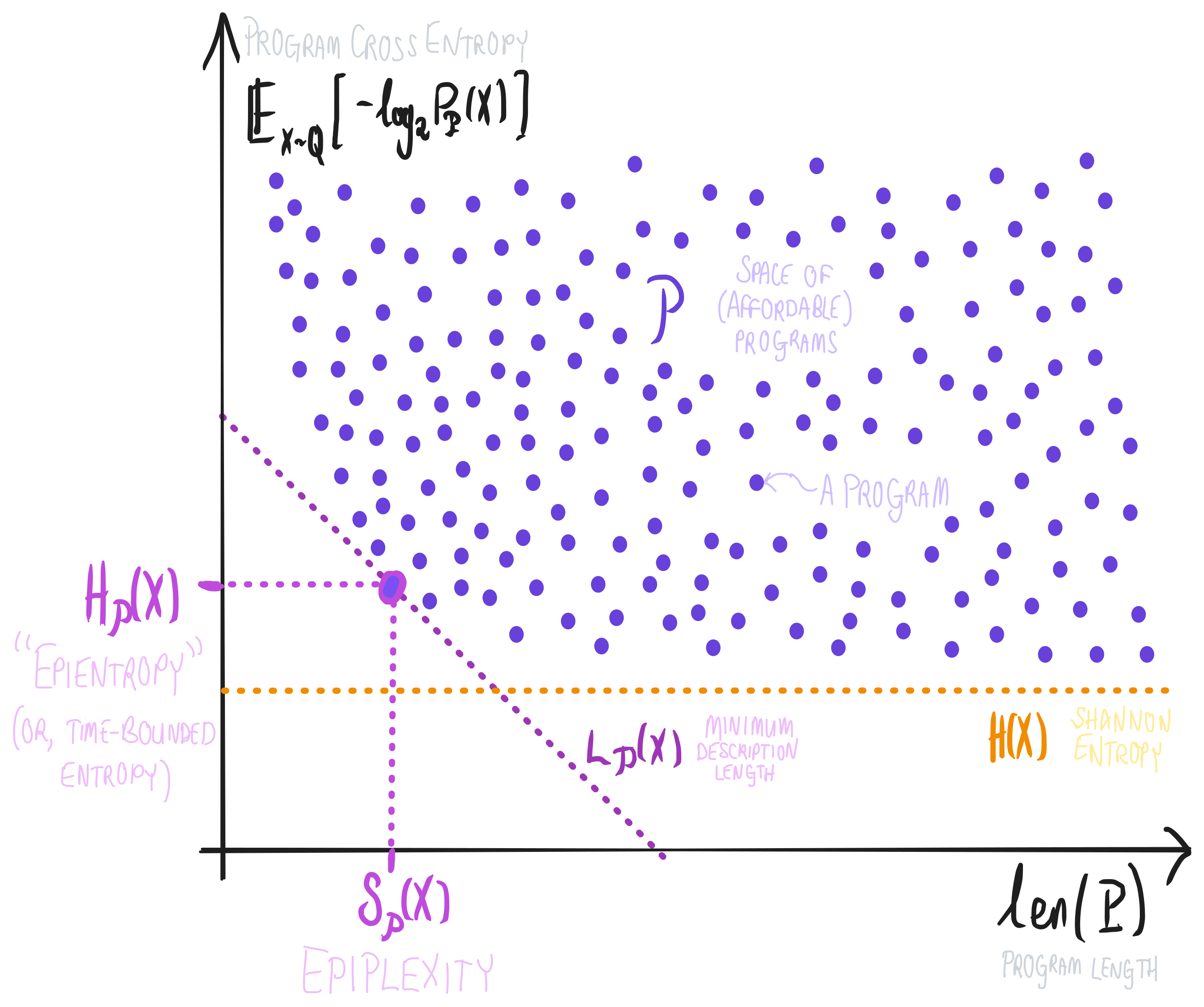
The specific shape of the point cloud $\mathcal{P}$ depends on which programs are included, on the universal Turing machine, and the variable $X$. However, we have the following basic bounds.

• Program length $\text{len}({\tt P}) \in \mathbb{N}$, in particular it’s non-negative.

  Zero itself may not be reached. Depending on the universal Turing machine, it can take a few bits minimum to encode a program (let alone a valid probabilistic model).

• Cross entropy $\mathbb{E}_{X \sim Q}\!\left[-\log_2 P_{{\tt P}}(X)\right] \geq \mathbb{E}_{X \sim Q}\!\left[-\log_2 Q(X)\right] = H(X) \geq 0$, using basic results from information theory ($H(X)$ denotes the entropy of $X$).

  The bound will be reached if and only if $P_{{\tt P}}= Q$ for some ${\tt P}\in P_{{\tt P}}$, otherwise we might approach the bound indefinitely (or as far as we can within our computational budget).

§Examples and basic properties of epiplexity

Now that we have a new pair of quantities, let’s see what we can do with them!

§§Uniform distribution

Lets say we have a variable $U$ distributed uniformly over $\{{\tt 0},{\tt 1}\}^{n}$. What is its epiplexity? The paper briefly describes this useful baseline.

First, assume that the uniform distribution over $\{{\tt 0},{\tt 1}\}^{n}$ is representable by some program ${\tt u} \in \mathcal{P}$. This should be true for most cases based on resource limitations, since the uniform density can be efficiently implemented (it’s a constant $2^{-n}$) and uniform sampling can be efficiently simulated (copy the first $n$ bits from the random tape). On any reasonable universal Turing machine this is probably one of the shortest and fastest valid probabilistic models implementable.

Assume without loss of generality that $\tt u$ is the shortest implementation of this probabilistic model in $\mathcal{P}$. Then we have: $$\begin{align*} L(U; {\tt u}) &= \text{len}({\tt u}) + \mathbb{E}_{U}\!\left[-\log_2 P_{\tt u}(U)\right] \\ &= \text{len}({\tt u}) + \mathbb{E}_{U}\!\left[-\log_2 2^{-n}\right] \\ &= \text{len}({\tt u}) + n. \end{align*}$$

In this case, we know this program achieves the minimum description length since we have minimised the cross entropy (it matches the entropy of $U$) and we have minimised the program length amongst affordable programs with that property by assumption. Therefore, we can read out the epiplexity and epientropy directly: $$S_\mathcal{P}(U) = \text{len}({\tt u}) \qquad H_\mathcal{P}(U) = n.$$

§§General upper bounds

While the uniform case was much easier to analyse than the general case, we can still leverage it to get a very general bound. Let $X \sim Q$ be arbitrary. Then, under the same assumptions on $\mathcal{P}$ and $\tt u$, we still have $$\begin{align*} L(X; {\tt u}) &= \text{len}({\tt u}) + \mathbb{E}_{X}\!\left[-\log_2 P_{\tt u}(U)\right] \\ &= \text{len}({\tt u}) + \mathbb{E}_{X}\!\left[-\log_2 2^{-n}\right] \\ &= \text{len}({\tt u}) + n. \end{align*}$$

This is not necessarily the minimum description length of $X$, but it does give us a general upper bound: $$\begin{align*} S_\mathcal{P}(X) + H_\mathcal{P}(X) &= L_\mathcal{P}(X) \\&= \operatornamewithlimits{\vphantom{arg\,}min}_{{\tt P}\in \mathcal{P}} L(X; {\tt P}) \\&\leq L(X; {\tt u}) \\&= \text{len}({\tt u}) + n. \end{align*}$$

This is “basic property (2)” noted in the paper. Unfortunately, in general we can’t extend this to a pair of bounds $S_\mathcal{P}(X) \leq \text{len}({\tt u})$ and $H_\mathcal{P}(X) \leq n$. The above bound only holds on the sum. Decreasing the description length may involve altering the trade-off between program length and cross entropy.

We can turn this upper bound on the sum into some basic upper bounds on each term, however, since we have lower bounds $0 \leq S_\mathcal{P}(X)$ and $0 \leq H(X) \leq H_\mathcal{P}(X)$: $$\begin{align*} H_\mathcal{P}(X) &\leq \text{len}({\tt u}) + n, \\ S_\mathcal{P}(X) &\leq \text{len}({\tt u}) + n - H(X) \leq \text{len}({\tt u}) + n. \end{align*}$$

We note that while none of these bounds are that powerful, they came easily: all we needed was a single program ${\tt u} \in \mathcal{P}$ with a known description length. We can re-apply the same reasoning as soon as we have any example program ${\tt P}\in \mathcal{P}$ (or any other bound on the description length): $$\begin{align*} S_\mathcal{P}(X) + H_\mathcal{P}(X) &\leq L(X; {\tt P}), \\ H_\mathcal{P}(X) &\leq L(X; {\tt P}), \\ S_\mathcal{P}(X) &\leq L(X; {\tt P}) - H(X) \leq L(X; {\tt P}). \end{align*}$$ When it comes to estimating epiplexity and epientopy in practical examples, we might be able to obtain reasonably tight bounds in some cases.

§§Relaxing the restrictions

Basic property (3) in the paper shows that relaxing the time restriction generally can only decrease the minimum description length. The reason is because this generally only makes more programs available for consideration, which can only expand the possibilities for minimisation.

This monotonicity property of the minimum description length can be generalised immediately to our more abstract setting by considering what happens if we generally add programs to the restricted class $\mathcal{P}$.

So, assume $\mathcal{P}' \supset \mathcal{P}$. Then we have $$\begin{align*} S_{\mathcal{P}'}(X) + H_{\mathcal{P}'}(X) &= L_{\mathcal{P}'}(X) \\ &= \operatornamewithlimits{\vphantom{arg\,}min}_{{\tt P}\in \mathcal{P}'} L(X; {\tt P}) \\ &\leq \operatornamewithlimits{\vphantom{arg\,}min}_{{\tt P}\in \mathcal{P}} L(X; {\tt P}) \\ &= L_{\mathcal{P}}(X) \\ &= S_{\mathcal{P}}(X) + H_{\mathcal{P}}(X). \end{align*}$$

Again, the bound does not tell us anything about whether the epiplexity or epientropy will decrease/increase individually, only that their sum will not increase if we expand our affordances. The optimal ratio between extracted structure and random information could potentially change in either direction.

§Recovering unbounded complexity and entropy

Epiplexity and epientropy were motivated by the desire to incorporate computational limitations into (algorithmic) information theory. If we remove the computational limitations, do we recover Kolmogorov complexity and Shannon entropy as epiplexity and epientropy respectively? Not quite, but they do show up in analogous positions.

First, we should assume the true underlying data distribution $Q$ is representable as a computable probabilistic model. For data we encounter in the real universe, this seems like a pretty safe bet (this is the so-called physical Church–Turing thesis).

Then, to remove all computational resource restrictions, let $\mathcal{P}$ represent all computable probabilistic models. By assumption, there is some ${\tt P}_\star \in \mathcal{P}$ such that $P_{{\tt P}_\star} = Q$. There will be many actually, define ${\tt P}_\star$ to be one of the shortest among them. We’ll define its length to be the Kolmogorov complexity of $X$, $K(X)$.

Then, the description length of $X$ via ${\tt P}_\star$ simplifies as follows: $$\begin{align*} L(X; {\tt P}_\star) &= \text{len}({\tt P}_\star) + \mathbb{E}_{X \sim Q}\!\left[-\log_2 P_{{\tt P}_\star}(X)\right] \\ &= K(X) + \mathbb{E}_{X \sim Q}\!\left[-\log_2 Q(X)\right] \\ &= K(X) + H(X) \end{align*}$$ where $H(X)$ is the Shannon entropy of $X$.

So we have found Kolmogorov complexity playing the role of a structure term, the first part of the two-part code, and Shannon entropy playing the role of a cross-entropy term, the second. This immediately gives us a bound on the (unbounded-compute) epiplexity and epientropy: $$S_\mathcal{P}(X) + H_\mathcal{P}(X) \leq K(X) + H(X).$$ To say more, we’d need to know that $L(X; {\tt P}_\star)$ is minimal. The problem is, it seems like it might not be minimal in general! $H(X)$ is as low as it’s possible to get the cross entropy term, but if we’re willing to raise the cross entropy term a little, we might sometimes be able to get away with a shorter program than $K(X)$ that still approximately matches $Q$.

§Independent sequences

A slightly more intricate example is the following. Suppose our random variable is actually a concatenation of independent and identically distributed substrings. I don’t believe this was discussed in the paper, but it’s a common assumption in learning, so it’s worth considering what we can say about this case. As I suspected, there turn out to be a few simple observations we can make.

§§Iterating variables

Formally, consider two random variables:

1. $X$, a random variable taking values in $\{{\tt 0},{\tt 1}\}^{n}$, distributed according to $Q \in \Delta(\{{\tt 0},{\tt 1}\}^{n})$; and

2. $X^m = X_1 X_2 \cdots X_m$ where $m > 1$ and each $X_i$ is an independent copy of $X$, that is, $X^m$ is a random variable taking values in $\{{\tt 0},{\tt 1}\}^{nm}$, distributed according to $Q^m \in \Delta(\{{\tt 0},{\tt 1}\}^{nm})$.

The goal of this section is to relate minimum description lengths, epiplexities, and epientropies across these two variables.

§§Iterating probabilistic models

One barrier is that each variable needs a different family of probabilistic models. Since these variables have different numbers of bits, they require probabilistic models with different type signatures. Let’s denote the affordable probabilistic models for $X$ as $\mathcal{P}_n$, and those for $X^m$ as $\mathcal{P}_{nm}$, where we use a subscript to indicate the relevant variable length.

One simple assumption we could make is to relate these program classes is to populate $\mathcal{P}_{nm}$ with iterated versions of the distributions in $\mathcal{P}_n$. Formally, given ${\tt P}\in \mathcal{P}_n$, define a probabilistic model ${\tt P}^m$ on $\{{\tt 0},{\tt 1}\}^{nm}$ based on the following density evaluation and sampling implementation:

• For density evaluation of a string $x_1 x_2 \cdots x_m \in \{{\tt 0},{\tt 1}\}^{nm}$, compute $P_{{\tt P}}(x_1)$, $P_{{\tt P}}(x_2)$, …, $P_{{\tt P}}(X_m)$ using ${\tt P}$, and return $P_{{\tt P}^m}(x_1 x_2 \cdots x_m) = \Pi_{i=1}^m P_{{\tt P}}(x_i)$.

• For sampling, generate samples $x_1, x_2, \ldots, x_m$ using ${\tt P}$ (consuming non-overlapping segments of the noise tape).

The result will be a probabilistic model and satisfy $P_{{\tt P}^m} = P_{{\tt P}}^m$. If we use a reasonable universal Turing machine, transforming ${\tt P}$ into ${\tt P}^m$ will only require a small number of bits to encode the iteration procedures and the constant $m \in \mathbb{N}$ (independent of the size of ${\tt P}$). Let’s adopt this assumption and call the constant $k_m$, such that we have $$\text{len}({\tt P}^m) = \text{len}({\tt P}) + k_m.$$ If we’re worried about time complexity, these constructions should only inflate the runtime of ${\tt P}$ polynomially in $n$ and $m$.

Let’s lift this to the set of programs $\mathcal{P}_n$. Define $\mathcal{P}_n^m$, a set of programs over $\{{\tt 0},{\tt 1}\}^{nm}$ containing $m$-iterated copies of the programs in $\mathcal{P}_n$: $$\mathcal{P}_n^m = \left\{\,{\tt P}^m \,\middle|\,{\tt P}\in \mathcal{P}_n\,\right\}.$$ We shall proceed by defining the restricted class $\mathcal{P}_{nm} = \mathcal{P}_n^m$. This might seem like a fairly restricted way to define an expanded class of programs. Note that except where noted, the following arguments work if we merely assume $\mathcal{P}_{nm} \supset \mathcal{P}_n^m$. This latter condition would be achieved by modestly expanding a time complexity bound, for example, as discussed above. Introducing more programs may lead to unexpected new minima, of course.

§§A basic upper bound

Intuitively, it seems like $X^m$ can’t have that much more (accessible) structural information than $X$, since one copy of $X$ already represents the full complexity of the distribution and $X^m$ just repeats that structure $m$ times. On the other hand, encoding multiple specific samples from the distribution means replicating the unpredictable structure multiple times. This all suggests that $X^m$ could have a similar epiplexity but a larger epientropy than $X$. As it turns out, this isn’t necessarily true, but we can at least turn this intuition into a description length bound, as follows.

Starting in the realm of $X$, suppose ${\tt P}_\star \in \mathcal{P}_n$ is a program achieving the minimum description length of $X$ (after breaking ties by shorter program length), such that $$\begin{align*} L_{\mathcal{P}_n}(X) &= L(X; {\tt P}_\star); \\ S_{\mathcal{P}_n}(X) &= \text{len}({\tt P}_\star); \\ H_{\mathcal{P}_n}(X) &= \mathbb{E}_{X\sim Q}\!\left[-\log_2 P_{{\tt P}_\star}(X)\right]. \end{align*}$$

By lifting ${\tt P}_\star \in \mathcal{P}_n$ to ${\tt P}_\star^m \in \mathcal{P}_{nm}$, we get the following basic upper bound on the minimum description length in the iterated case. $$\begin{align*} S_{\mathcal{P}_{nm}}(X^m) + H_{\mathcal{P}_{nm}}(X^m) &= L_{\mathcal{P}_{nm}}(X^m) \\ &\leq \text{len}({\tt P}_\star^m) + \mathbb{E}_{X^m\sim Q^m}\!\left[-\log_2 P_{{\tt P}_\star^m}(X^m)\right] \\ &= (\text{len}({\tt P}_\star) + k_m) + \mathbb{E}_{X^m\sim Q^m}\!\left[-\log_2\left( \prod_{i=1}^m P_{{\tt P}_\star}(X_i) \right)\right] \\ &= \text{len}({\tt P}_\star) + k_m + m \mathbb{E}_{X \sim Q}\!\left[-\log_2 P_{{\tt P}_\star}(X)\right] \\ &= S_{\mathcal{P}_n}(X) + k_m + m H_{\mathcal{P}_n}(X). \end{align*}$$ The result is a satisfyingly interpretable bound on the description length in the iterated case! Look:

• In the first part of this two-part code (via ${\tt P}_\star^m$), namely the first two terms of the bound, we’re proposing to encode the program ${\tt P}_\star$ plus a small amount of additional structure ($k_m$) required to specify that it is being iterated.

• In the second part of the two-part code, we see that we have to pay $m$ times the cost of coding a single example’s remaining bits. This makes sense, since there are $m$ random draws to be had.

The satisfying part is that while we paid the entropy encoding cost repeatedly, we didn’t have to do this for the program length. As long as $m$ is large or $k_m$ is otherwise relatively small, we’re way out-competing the naive coding approach of separately coding each sample along with its own copy of the program.

§§Weighted minimum description length

Can we do better? Is this upper bound tight? Assuming $\mathcal{P}_{nm} = \mathcal{P}_n^m$, the bound might be tight in some cases, depending on $\mathcal{P}_n$. But, it could easily be suboptimal, for the following reason.

Formally, assuming $\mathcal{P}_{nm} = \mathcal{P}_n^m$, we can perform a similar decomposition of the description length for all programs ${\tt P}^m \in \mathcal{P}_{nm}$ as we did for ${\tt P}_\star^m$: $$\begin{align*} L(X^m; {\tt P}^m) &= \text{len}({\tt P}^m) + \mathbb{E}_{X^m\sim Q^m}\!\left[-\log_2 P_{{\tt P}^m}(X^m)\right] \\ &= (\text{len}({\tt P}) + k_m) + \mathbb{E}_{X^m\sim Q^m}\!\left[-\log_2\left( \prod_{i=1}^m P_{{\tt P}}(X_i) \right)\right] \\ &= \text{len}({\tt P}) + k_m + m \mathbb{E}_{X \sim Q}\!\left[-\log_2 P_{{\tt P}}(X)\right]. \end{align*}$$

We can thus reduce the problem of minimising description length of $X^m$ over $\mathcal{P}_{nm}$ to a minimisation problem involving $X$ and $\mathcal{P}_n$. The result is subtly different from the problem of minimising description length of $X$. We can ignore that the objective has an extra $k_m$ term. We assumed $k_m$ does not vary with ${\tt P}$. Therefore, it can’t change where the minimum is: $$\operatornamewithlimits{arg\,min}_{{\tt P}^m \in \mathcal{P}_{nm}} L(X^m; {\tt P}^m) = \operatornamewithlimits{arg\,min}_{{\tt P}\in \mathcal{P}_{n}} \big\{ \text{len}({\tt P}) + m \mathbb{E}_{X \sim Q}\!\left[-\log_2 P_{{\tt P}}(X)\right] \big\}.$$ The important difference from the original objective is that this objective has a different coefficient on the cross entropy term. This is a meaningful change. It means we should think of increases in cross entropy as more costly than increases in program length when balancing the two. Equivalently, we could imagine down-weighting the program complexity versus the cross entropy.

Intuitively, the interpretation of this coefficient is that the need to encode samples from $m$ copies of $X$ creates a greater incentive to export structure into the first part of the two-part code. Specifically, we previously would have declined the option to add one bit to reduce the cross entropy by a fractional $k \in (1/m, 1]$ bits. In the iterated case, this is a good deal, as we get to repeat that saving $m$ times leading to an overall saving of $mk > 1$ bits.

If there is a program ${\tt P}\in \mathcal{P}_n$ that offers that kind of trade, then it will beat ${\tt P}_\star$ on description length in the iterated case. However, at least we can tell this will be the case by analysing the single-variable case, as long as we search for the best program with a re-weighted objective.

§§Allowing more programs

If we relax the strong assumption that $\mathcal{P}_{nm} = \mathcal{P}_n^m$, this connection breaks down. It might be the case that these iterated probabilistic models not available for modelling $X^m$. Or, there might be more programs to choose from that offer better tradeoffs.

The paper normally considers a computational budget to be expressed as an increasing function of the number of bits in the data. By this idea, the increased size of $X^m$ justifies giving $\mathcal{P}_{nm}$ access to programs that require more computational resources. Doing so might take us into a regime where new structural information becomes efficiently extractable from each sample, allowing better compression of individual samples, increasing program length while decreasing per-sample cross entropy. It’s also possible that new options for substantially decreasing program length while increasing per-sample cross entropy, or even opportunities to decrease both program length and per-sample cross entropy, could appear.

Another possibility worth considering is that it might be possible to take advantage of programs that don’t take full advantage of iteration. This is a bit hard to imagine, since iteration is likely to be such a salient structural element of the problem, and it might be optimal for most reasonable universal Turing machines. However, I think it might be possible to construct some kind of counterexample where we can save a lot on program length by approximating the iterative structure with some slightly out-of-phase iteration that leads to nearly as low cross entropy.

§Breaking ties

Epiplexity is defined as the length of the shortest programs involved in optimal two-part codes. It was necessary to say “the shortest” programs even though we already said “optimal two-part codes” because optimal two-part codes might be based on programs with different lengths. Refer to these situations as ties. In this section, let’s explore ties and consider different ways of breaking them.

§§What are ties?

What would it mean for there to be two optimal codes with different program lengths? Let’s break that down.

We’d want two programs ${\tt P}_1, {\tt P}_2 \in \mathcal{P}$ such that $${\tt P}_1, {\tt P}_2 \in \operatornamewithlimits{arg\,min}_{{\tt P}\in \mathcal{P}} \big\{ \text{len}({\tt P}) + \mathbb{E}_{X \sim Q}\!\left[-\log_2 P_{{\tt P}}(X)\right] \big\}.$$ In particular, it must be that $$\text{len}({\tt P}_1) + \mathbb{E}_{X \sim Q}\!\left[-\log_2 P_{{\tt P}_1}(X)\right] = \text{len}({\tt P}_2) + \mathbb{E}_{X \sim Q}\!\left[-\log_2 P_{{\tt P}_2}(X)\right] .$$ Equivalently, $$\mathbb{E}_{X \sim Q}\!\left[-\log_2 P_{{\tt P}_1}(X)\right] = \mathbb{E}_{X \sim Q}\!\left[-\log_2 P_{{\tt P}_2}(X)\right] + (\text{len}({\tt P}_2) - \text{len}({\tt P}_1)) .$$ That is, if ${\tt P}_2$ is longer by a number of bits, it must offer a cross entropy lower by exactly that many bits. Since these bits come out of the cross entropy and go into the program length, this is a neutral tradeoff from a minimum description length perspective, which is why both codes are considered optimal.

§§Toy example of a tie

Do ties even exist? I don’t know how common they would be in practice, but it’s easy enough to fabricate them in a toy example.

Consider a very simple problem with $n=1$ and $X \sim \text{Bernoulli}(q)$ for some hyper-parameter $q \in (0,1)$. Imagine there are only two programs in our set of probabilistic models, $\mathcal{P}= \{{\tt P}_1, {\tt P}_2\}$, respectively representing Bernoulli distributions with parameters $p_1, p_2 \in (0,1)$ with program lengths $\ell_1, \ell_2$.

In this simple case, we can compute $$\begin{align*} L(X; {\tt P}_i) &= \text{len}({\tt P}_i) + \mathbb{E}_{X \sim \text{Bernoulli}(q)}\!\left[-\log_2 P_{{\tt P}_i}(X)\right] \\ &= \ell_i - q \log_2 p_i - (1 - q) \log_2 (1 - p_i). \end{align*}$$ Equating $L(X; {\tt P}_1) = L(X; {\tt P}_2)$, we can solve for $q$ to produce a tie: $$q = \frac{ \ell_2 - \ell_1 + \log_2 \frac{1 - p_1}{1 - p_2} }{ \log_2 \frac{p_2}{1-p_2} - \log_2 \frac{p_1}{1 - p_1} }.$$

§§Why break for less structure?

If we ever were to face this situation, the paper says we should break for the smaller program length when defining epiplexity. Why might we want to define epiplexity in terms of the smaller program?

This choice can’t be justified based on the minimum description length framework, since it’s neutral to this trade-off by construction. Let’s explore some possible justifications. On the one hand, the smaller program is appealing for a number of reasons:

• First, we could appeal to Occam’s razor, saying that the smallest model that explains the data is the better one. Here we aren’t exactly explaining the data, we’re compressing it using a two-part code, but we might coarsely apply Occam’s razor in the form “all else equal, smaller models are better,” and that points to the shorter program.

• Alternatively, let’s return to the original motivation of asking the question, “how much structural information can we profitably extract from data?” We might say that if you are converting data bits into program length at a 1:1 rate, you’re not extracting structure at all, you’re just memorising bits. You should stop extracting structure as soon as you get to the point where you can no longer shrink the second part of the code strictly more than you have to increase the first. That’s the shorter program. (Thanks to Joan Velja for this perspective!)

On the other hand, I can see a way of arguing for the opposite perspective in each case.

• Occam’s razor be damned: cross entropy is loss. Loss is bad, and our goal when modelling should be to minimise it. All else being equal, we should reduce loss, not program length. Therefore, go for the longer program.

• It isn’t always possible to memorise bits of a random variable. These bits aren’t exactly entropy either. Maybe 1:1 structure is still structure, and if we’re trying to count structure, we should still count these bits. Therefore, go for the longer program.

I don’t know what to make of this. It seems like maybe both answers could be valid.

§§Alternative tie-breakers

Maybe we should appeal to a completely outside perspective to resolve the tie.

We could consider adding a third axis to minimise/maximise:

• Maybe we should choose the most efficient program among the programs generating optimal codes. Or some combination of efficiency and program length.

• Maybe we should choose appeal not only to the expected cross entropy, but to the variance in coding costs associated with different coding schemes, or other downside-risk-minimising objectives like expected shortfall, in case we are worried about getting unlucky when it comes time to actually code samples of $X$ with the optimal code designed for the distribution.

• Ultimately, if we want to leverage the bounded-computation perspective offered by epiplexity to understand deep learning, the right way to break the tie might be an empirical question. What version of the definition more aptly plays a role in attempts to explain deep learning phenomena?

§§Dissolving the tie

We don’t necessarily have to break the tie. Maybe the different options are genuinely telling us different things about the problem.

We could perhaps acknowledge this with two definitions. The shortest program length could be called the lower epiplexity, and the longest program length the upper epiplexity. Conversely, we could talk about the respective complement quantities, the upper and lower epientropy.

Or maybe, we could separate the minimum description length of our variable into three quantities instead of just two. We could separately count the (lower) epiplexity, the (lower) epientropy, and also the remaining, intermediate bits that can be exchanged between program length and cross entropy at a 1:1 rate. However, we should recognise that not all positions along this equilibrium region need be realisable.

My conclusion overall is that it seems fine for now to define epiplexity in terms of the paper’s tie-breaking rule, but it’s good to be aware that we are doing this, and be ready to refer to these more refined concepts if the need arises in the future.

§Conclusion

I like the epiplexity framework. It seems like a sensible step on the road from algorithmic information theory towards a theory of information and learning that takes bounded resources into account. This is part of an exciting shift in the field of algorithmic information theory that is as deep as the split between computability and complexity theory in theoretical computer science. This analogy is not drawn by coincidence, as indicated by the extent to which the paper draws on complexity and cryptography theory in its theoretical results. In fact, we have individual figures like Levin whose work has been at the foundation of complexity theory (with the Cook–Levin theorem) and also the foundation of this new direction (with the invention of Levin complexity, another formulation of resource-limited algorithmic information theory). I am glad I took the time to understand the definition of epiplexity thoroughly. This has generated some interesting theoretical questions about potential loopholes in the observer’s computational budget, and idea to change the definitions to fix them. Suffice it to say, I am going to ponder these and may write about them in a future post.

I’m excited to continue reading and reflecting on the paper’s empirical sections, too. If this approach can really shed light on some of the stunning phenomena driving the AI revolution, then that will be light sorely needed indeed. In this regard, I am less concerned about the potential gaps in the framework. Pragmatically speaking, I think it’s an acceptable strategy to enrich our theories on an as-needed basis. The field of machine learning has spent a long time under the faint guiding glow of resource-unlimited algorithmic information theory, throwing around terms like Kolmogorov complexity and Solomonoff induction. Let’s see whether epiplexity can show us the way to new, fruitful experiments and empirical insights. Maybe the shadowy parts aren’t obscuring anything important, in which case they won’t turn out to matter at the end of the day. Or maybe they will turn out to be important—if this new light runs out on us, we can invest again in improving our theory.